Info:

Learn to transform your Excel document to fit the guidelines for data used in Valsight with Power Query!

Overview

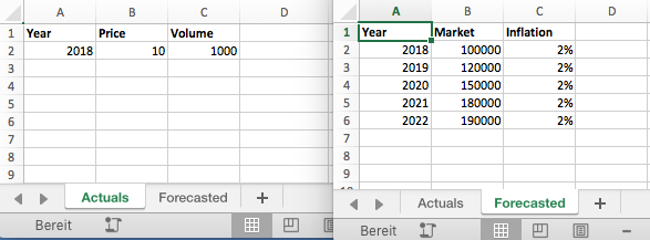
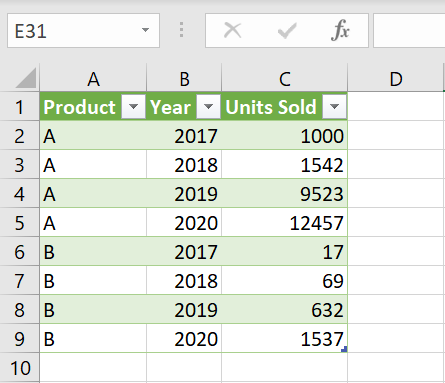
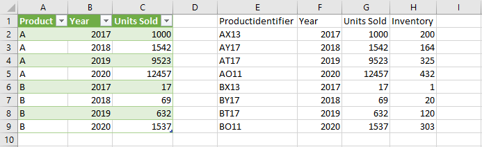
Data sources uploaded to Valsight need to be correctly formatted as shown in the picture below.

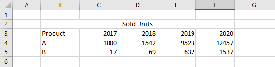
If you have an Excel document that is not following those guidelines (e.g. the document in the picture below), there is an easy way of changing it into the correct format using Excel Power Query.

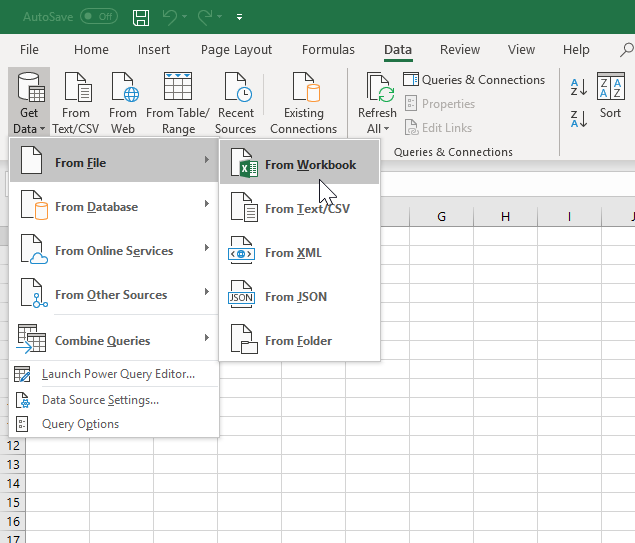
Create an empty Excel document and select ‘Data’ → ‘Get Data’  → ‘From File’ → ‘Excel Worksheet’. Now select the file that contains the desired data.

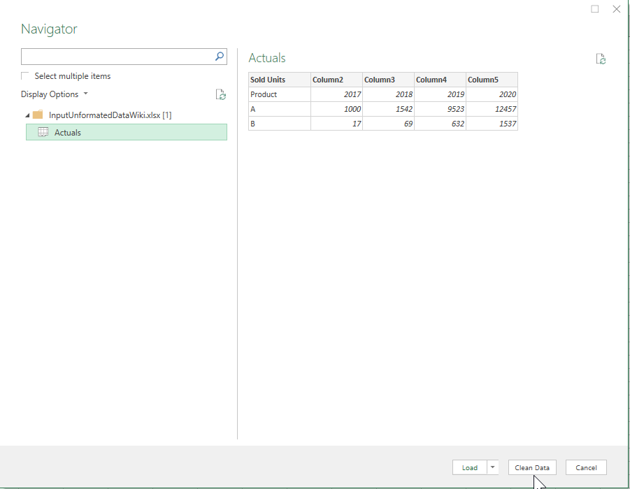
Excel automatically imports the data. Now select ‘Clean Data’ to change the data structure in the Power Query-Editor.

Changing the Data Structure

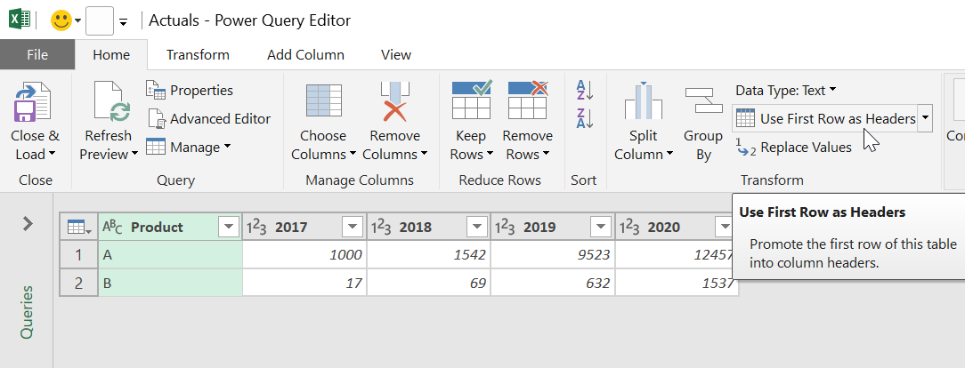
In this case, select ‘Use First Row As Headers’ to properly title the columns. In general, use the suitable tool for your need offered by the Power Query-Editor (e.g. “Remove Rows/Columns”, “Split Column”, …) to transform your table.

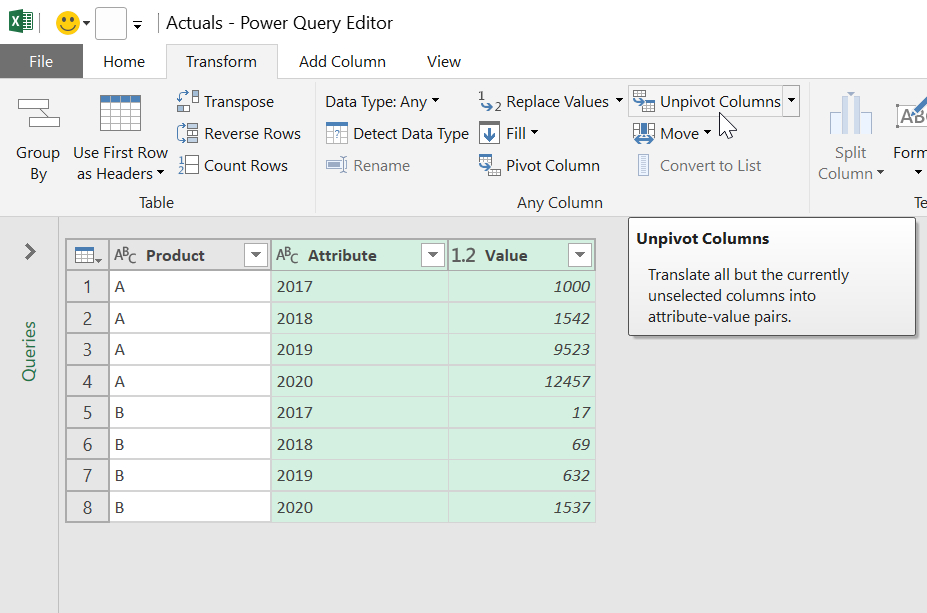
The next step is to select all the columns containing data. In this case this means selecting the columns ‘2017’, ‘2018’, ‘2019’ and ‘2020’.  Afterward, click ‘Transform’ → ‘Unpivot Columns’.

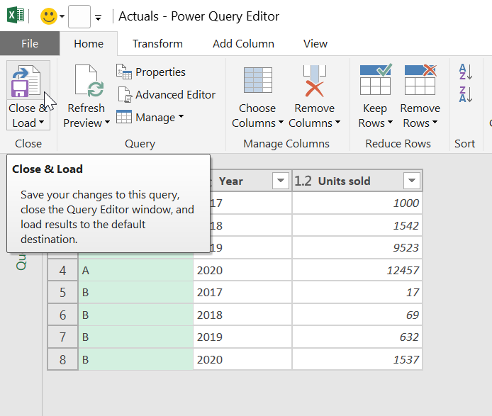
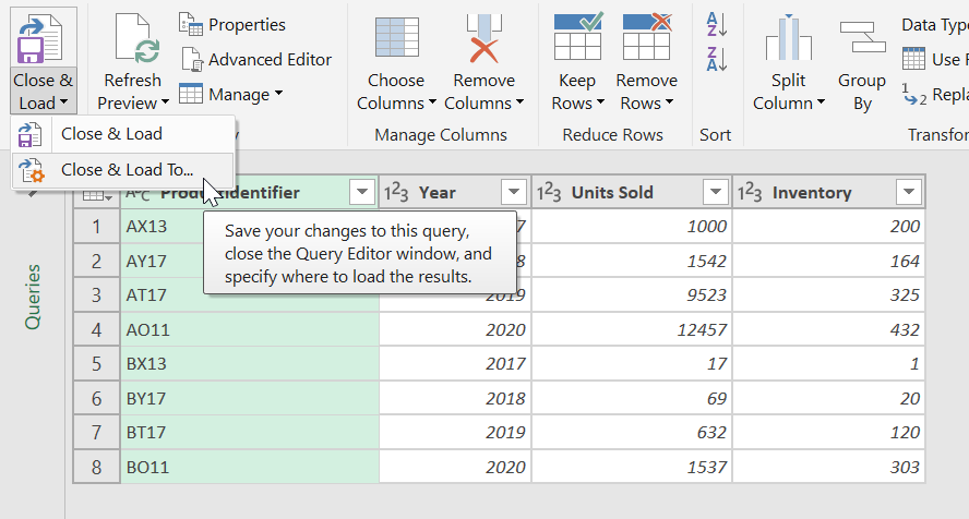
Now the only thing left to do is rename the columns by double clicking on their title and to ‘close & load’.

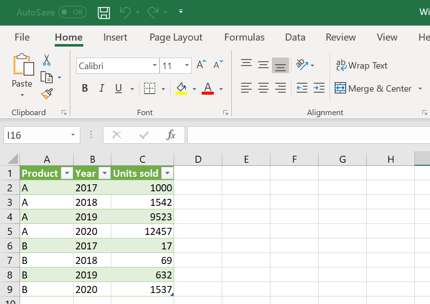
Congratulations, you have successfully restructured your data. The resulting worksheet is now linked to the original document.

Import Data via Direct Filepath

Power Query offers the opportunity to connect the desired file path directly, to receive the matching data.

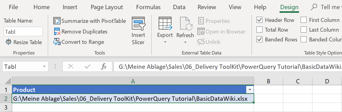
The first task is to create a table with one column and one row. You have to name the column (e.g. “Product”) and the table (e.g. “Tabl”) to reference them later.

Now you write down the file path, which leads to the desired, data, to the only cell.

Afterward, you open the Power Query-Editor containing the advanced Editor, as seen below.

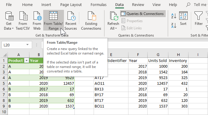
Select your table and go ‘Data’ → ‘From Table/Range’ → ‘Home’ → ‘Advanced Editor’.

There you type down the following command. Be careful to reference your table and column name correctly, furthermore the sheet reference ({[Item=“Tabelle1”,..) of the desired data.

let

    my_source= Excel.Workbook(File.Contents(Text.From(List.First(Table.Column(Excel.CurrentWorkbook(){[Name="Tabl"]}[Content], "Product")) )), null, true),
    Sheet1_Sheet = my_source{[Item="Tabelle1",Kind="Sheet"]}[Data]
in
    Sheet1_Sheet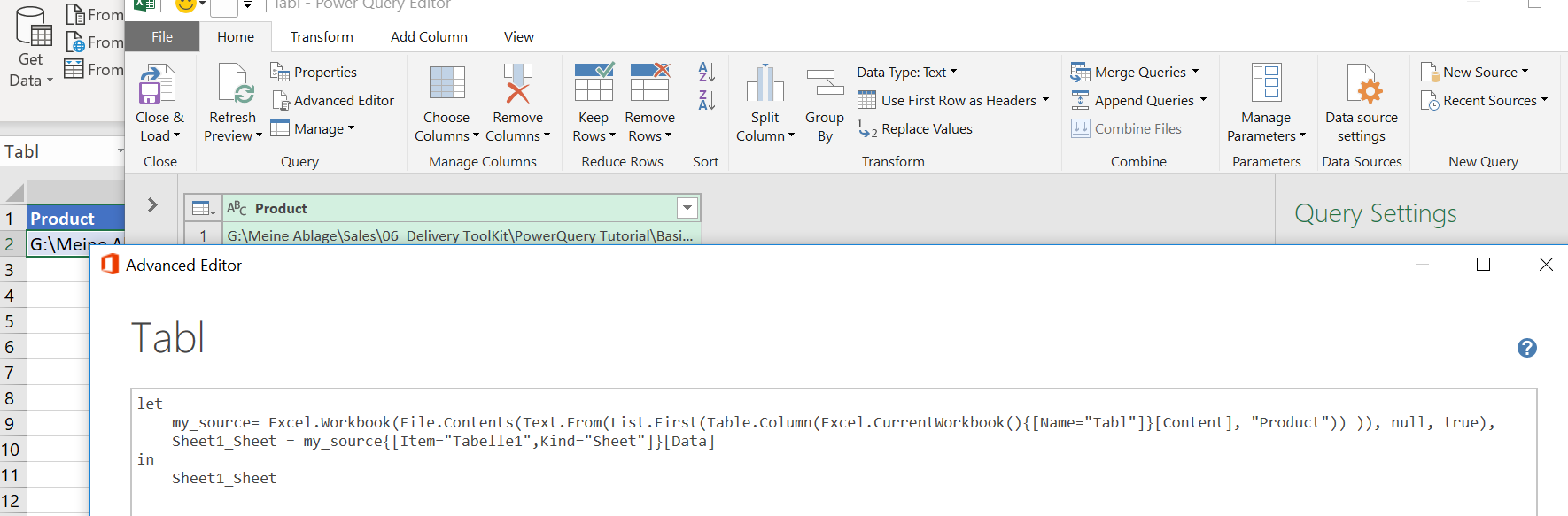

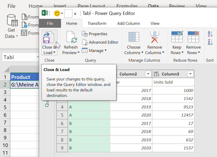
If you referenced everything correctly, the preview of the data becomes visible.

Just do “Close & Load” to finish the process.

It’s done, you created a new sheet that contains the data.

A change or expansion of the referenced data will be adapted automatically.

Mapping

Let’s continue with the given data table. To expand or substitute the given data you can use the “Join” Functions of Power Query.

You can add the additional data in different ways, usually by copying/pasting or manually.

Afterward, you convert the data into a second table by selecting the desired data and selecting ‘From Table/Range’.

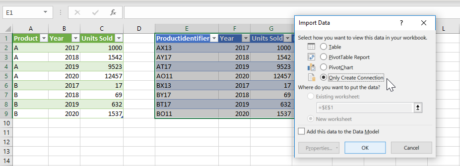
Now you close it and import it as a connection only.

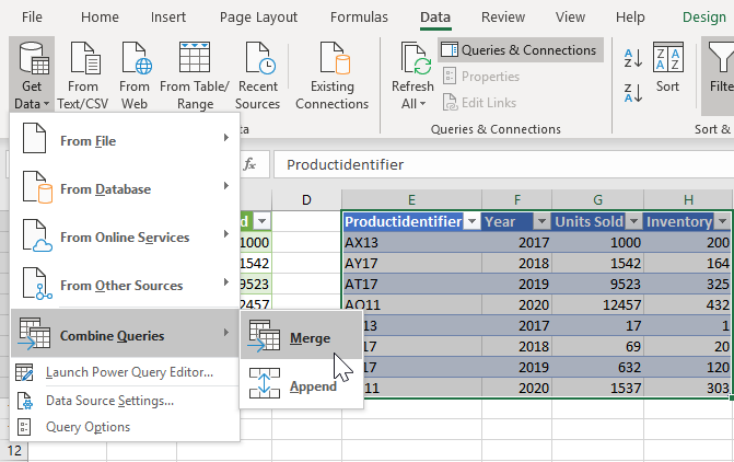
By selecting ‘Data’ → ‘Get Data’  → ‘Combine Query’ → ‘Merge’ you reach the Merge Window.

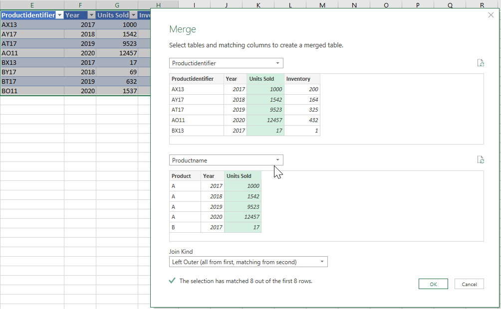
There you select for each field one of the given data tables and mark the matching columns.

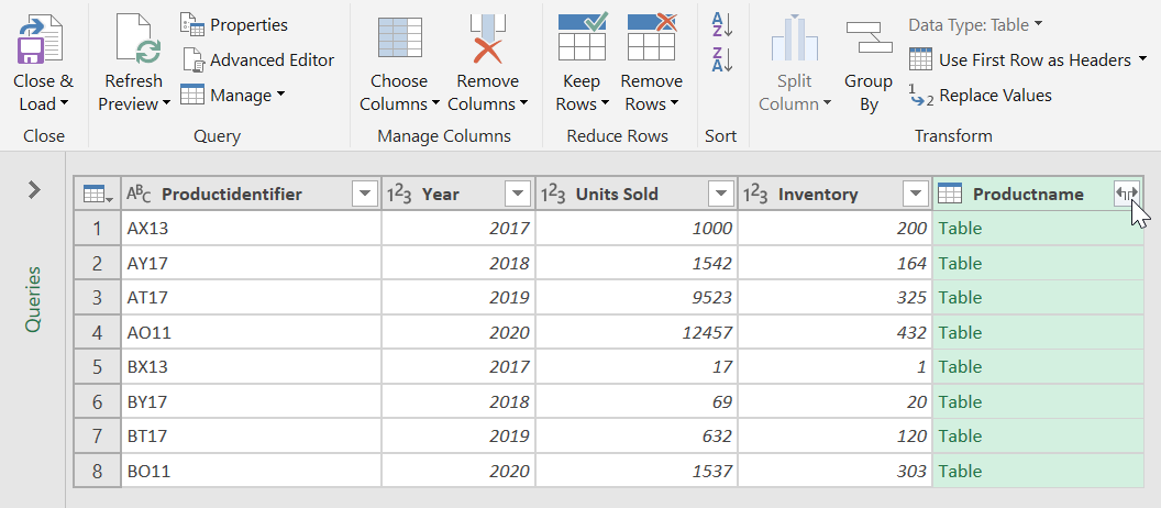
You can process with the resulting Power Query depending on your needs. To remove the “Productname” information you only need to delete the column.

For more options push the shown icon and choose the information you want to keep.

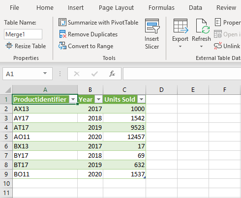
Now, select ‘Close & Load’ and your new data table is ready.

Transforming a Date to a Valsight Month

= Table.AddColumn(#"Geänderter Typ1", "TEst", each Text.Combine(
  {
    Number.ToText(Date.Year([Month])),
    "-",
    Number.ToText(Date.Month([Month]),"00")
  }))